Binary Outcomes, Risk Aversion, and Sorites Paradox (Part I)

Over the past few weeks, I’ve been diving deep into the world of coin tosses. It’s a simple yet fascinating experiment: you have a fair coin, and by “fair,” we mean that it has an equal chance of landing on either side—heads or tails. Starting with a fair coin is standard practice, especially in textbook examples, because it gives us a clean 50/50 chance for each outcome. In other words, the probability of getting heads is the same as getting tails, at 50% each.

Every time you flip the coin, you’re guaranteed to get either heads or tails. Of course, we can’t completely ignore the slim chance of the coin landing on its edge, which technically gives us a third possible outcome. But I’ll skip that for now.

Let’s keep our focus on the two possible outcomes of a single flip of a fair coin—heads or tails. The outcome is binary, and there’s something quite satisfying about that simplicity. In a world where complexity often leads to confusion, binary logic provides a clear, straightforward path to making decisions or drawing conclusions. By reducing possibilities to just two distinct outcomes, it simplifies complex situations, making them more manageable and easier to grasp.

Let’s dive into a few experiments to better grasp the concept of coin flipping. For simplicity, let’s consider the coin landing on heads as our desired outcome. Now, with a fair coin—where each toss is independent of any other—the calculations unfold like this:

1. The probability of getting one head in a single toss = 50%

2. The probability of getting two heads in two tosses = 50% * 50% = 25%

3. The probability of getting three heads in three tosses = 50% * 50% * 50% = 12.5%

4. And so on

As the number of tosses increases, we can model outcomes using what’s known as a binomial distribution. This type of distribution helps us predict how often a specific outcome, like landing on heads, will occur over a series of trials. For example, if you flip a coin 10 times and want to know the likelihood of getting exactly 0, 1, 2, …, or 10 heads, the binomial distribution is your go-to tool.

The formula for a binomial distribution is as follows:

Here, (n choose k) is the binomial coefficient, which calculates how many different combinations of k successes can occur in n trials. The term p represents the probability of the desired outcome (heads, in our case), while (1−p) represents the probability of the undesired outcome (tails).

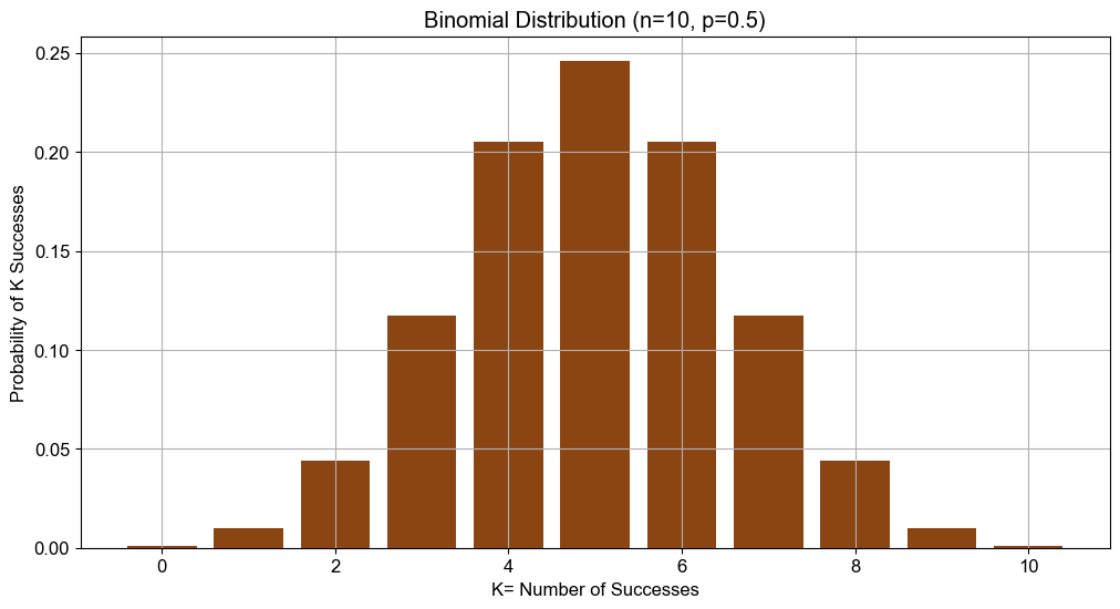
For a fair coin where the probabilities of heads and tails are equal (p = 0.5), the expression p^(k)*(1−p)^(n−k) simplifies to p^n, meaning the probability is driven largely by the binomial coefficient. Below is a simple illustration of what this looks like for 10 trials with varying outcomes of k:

You’ll observe that the distribution creates a symmetric, bell-shaped curve, peaking at 5 heads.

Binary thinking can similarly provide clarity when deciding whether to take the next step. The approach involves breaking down complex tasks into simpler, more manageable components.

For instance:

Goal: I want to learn probability theory (a broad and open-ended challenge).

1. Breaking it down: To learn probability theory, I need to study various resources (which is still too broad).

2. Refinement: I should select a specific book (a more focused and actionable task).

3. Further Breakdown: Have I read a page in the book? This binary question—essentially a “yes” or “no”—guides the next action.

In relation to our coin toss experiment, reading a page is akin to achieving a success. Initially, you might assume a 50% probability of success, similar to a coin toss with equal chances. While one might argue that each success increases your likelihood of future success, this introduces a complication: in a binomial distribution, each trial is independent.

To address this, consider that the probability of success might increase in discrete increments rather than continuously. We discussed this idea in our article “Continuity, Jumps, and Measuring Progress”. For example, after reading 1000 pages, your probability of successfully reading the next page (for the next 1000 pages) could rise from 50% to 60%. In our terms, this represents a “leveling up.”

But how does this affect our binomial distribution? When p and (1−p) are not equal—say, when the probability of success is 90% —the distribution becomes skewed.

Skewness measures the asymmetry of a distribution around its mean.

1. Positive Skew (Right Skew): A distribution with positive skewness has a longer or fatter right tail, meaning there are a few unusually high values that pull the mean upwards.

2. Negative Skew (Left Skew): A distribution with negative skewness has a longer or fatter left tail, indicating that a few unusually low values pull the mean downwards.

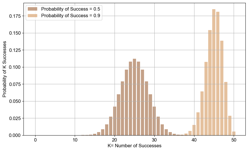
To illustrate this, I’ve provided two histograms below: one showing a 50% success rate and another with a 90% success rate, with the number of trials increased from 10 to 50 to clarify the point:

This is crucial for our discussion. The charts reveal that as the probability of success increases, the distribution with a 90% success rate becomes negatively skewed.

Although the mean outcome is higher in this distribution, it has a longer left tail, suggesting that even with a higher average success rate, there are still significant risks of negative outcomes. To me, this represents a shift in the psychological perception of our player who wants to successfully keep moving forward: while they might have a higher mean of overall success, they also face increased downside risks, which could heighten risk aversion despite a lower expected dispersion of outcomes (as shown by the coefficient of variation in Table 2).

For a fixed number of trials (n=50), I’ve included mean, standard deviation, coefficient of variation, and skewness across different probabilities of success in Table 2 below:

Additionally, Table 3 illustrates how skewness varies with both probability of success and the number of trials. As the number of trials increases, skewness approaches zero, reflecting the tendency for binomial distributions to approximate a normal distribution with a large number of trials.

However, for our purposes, it’s reasonable to assume that for any given goal, we typically encounter a limited number of trials and, if successful, generally find ourselves in the top-right section of Table 3 with negative skewness.

This suggests that higher-performing agents (represented via a distribution with probability of success greater than 50%), despite having a better average outcome, might experience greater risk aversion due to the higher potential for negative surprises.

Thus, in practical terms, a higher probability of success does not necessarily equate to lower perceived risk; rather, it can lead to an increased sensitivity to adverse outcomes. This shift in risk perception highlights the interplay between expected success and the psychological impact of potential losses.

In Part II, we will delve into some of the nuances that we have chosen to overlook in this discussion. Specifically, we will examine the limitations of binary outcomes through the lens of Sorites Paradox, explore the complexities introduced by embedding learning rates as proxies for probability of success using a Poisson distribution, and investigate what happens when learning rates fluctuate continuously rather than changing at discrete intervals.